![]()
![]()
The phenor R package is a phenology modelling framework in R. The framework leverages measurements of vegetation phenology from four common phenology observation datasets combined with (global) retrospective and projected climate data (see below).
The package curently focusses on North America and Europe and relies heavily on Daymet and E-OBS climate data for underlying climate driver data in model optimization. The package supports global gridded CMIP6 forecasts scenarios using the ECMWF Copernicus CDS service.
Phenological model calibration / validation data are derived from: - the transition dates derived from PhenoCam time series through the phenocamr R package - the MODIS MCD12Q2 phenology product using the MODISTools R package - the Pan European Phenology Project (PEP725) - the USA National Phenological Network (USA-NPN) - custom CSV based datasets
We refer to Hufkens et al. (2018) for an in depth description and worked example of the phenor R package. All code used to generate the referenced publication is provided in a separate github repository. Please refer to this paper when using the package for modelling efforts.
Keep in mind that some of the scripts will take a significant amount of time to finish. As such, some data generated for the manuscript is included in the manuscript repository. Some scripts generate figures and summary statistics on precompiled datasets rather than clean runs, when available. Furthermore, due to licensing issues no PEP725 data is included and some scripts will require proper login credentials for dependent code to function properly. Similarly, a download routine is not provided for the E-OBS data as to adhere to their data sharing policy and their request to register before downloading data.
Installation
- for the original package as described in the paper use release v1.0. Note that CMIP5 via NASA NEX has been deprecated in this releaseTo install the latest stable release of the toolbox in R run the following commands in a R terminal
if(!require(remotes)){install.packages("remotes")}
remotes::install_github("bluegreen-labs/phenor@v1.3.1")
library(phenor)
The development release can be installed by running
if(!require(remotes)){install.packages("remotes")}
remotes::install_github("bluegreen-labs/phenor")
library(phenor)
Download a limited subset of the data described in Richardson et al. (2017) from github or clone the repository:
git clone https://github.com/bluegreen-labs/phenocam_dataset.gitor download the full dataset from the ORNL DAAC.
Use
Example code below shows that in few lines a modelling exercise can be set up. You can either download your own data using the phenocamr package and format them correctly using pr_fm_phenocam()
# The command below downloads all time series for deciduous broadleaf
# data at the bartlett PhenoCam site and estimates the
# phenophases. By default data are downloaded into tempdir() (the
# temporary directory)
library(phenocamr)
phenocamr::download_phenocam(
  veg_type = "DB",
  roi_id = "1000",
  site = "bartlett",
  phenophase = TRUE
  )

# process phenocam transition files into a consistent format
phenocam_data <- pr_fm_phenocam(tempdir())
Alternatively you can use the included data which consists of 370 site years of deciduous broadleaf forest sites as included in PhenoCam 1.0 dataset (Richardson et al. 2017) precompiled with Daymet climate variables. The file is loaded using a standard data() call or reference them directly (e.g. phenocam_DB).
# load the included data using
data("phenocam_DB")
Model development, and parameter estimation
The gathered data can now be used in model calibration / validation. Currently 17 models as described by Basler (2016) are provided in the pacakge. These models include: null, LIN, TT, TTs, PTT, PTTs, M1, M1s, PA, Pab, SM1, SM1b, SQ, SQb, UN, UM1, PM1 and PM1b models as described in Basler (2016). In addition three spring grassland (pollen) phenology models: GR, SGSI and AGSI are included as described in Garcia-Mozo et al. 2009 and Xin et al. 2015. Finally, one autumn chilling degree day model (CDD, Jeong et al. 2012) is provided. Parameter values associated with the models are provided in a separate file included in the package but can be specified separately for model development.
# comma separated parameter file inlcuded in the package
# for all the included models, this file is used by default
# in all optimization routines
path <- sprintf("%s/extdata/parameter_ranges.csv",path.package("phenor"))
par_ranges <- read.table(path,
                        header = TRUE,
                        sep = ",")
Your own model development can be done by creating similar functions which take in the described data format and parameters. Below is the function to optimize the model parameters for the TT (thermal time) model using Generalized Simulated Annealing (GenSA). Uppper and lower constraints to the parameter space have to be provided, and in case of GenSA initial parameters are estimated when par = NULL.
# optimize model parameters
set.seed(1234)
optim.par <- pr_fit_parameters(par = NULL,
                          data = phenocam_data,
                          cost = rmse,
                          model = "TT",
                          method = "GenSA",
                          lower = c(1,-5,0),
                          upper = c(365,10,2000))
After a few minutes optimal parameters are provided. We can use these now to calculate our model values and some accuracy metrics.
# now run the model for all data in the nested list using the estimated parameters
modelled <- pr_predict(data = data, par = optim.par$par)
Easy model calibration / validation can be achieved using the model_calibration() and model_comparison() functions. Which either allow for quick screening for model development, or the comparison of a suite of models (using different starting parameters). I hope this gets you started.
Model projections and spatial data
The package allows you to download gridded CMIP5 forecast data from the NASA Earth Exchange global daily downscaled climate projections project. Hindcast data are provided for global NASA Earth Exchange, Berkeley Earth, E-OBS and gridded Daymet data (at 1/4th degree, 1 degree, 1/4th degree, 1km resolutions respectively).
# running data on spatial data (determined by the class assigned by
# various format_*() routines) will return a spatial object (raster map)
map <- pr_predict(data = spatial_data, par = optim.par$par)
An example of NASA Earth Exchange CMIP5 output and gridded Daymet data is provided below.
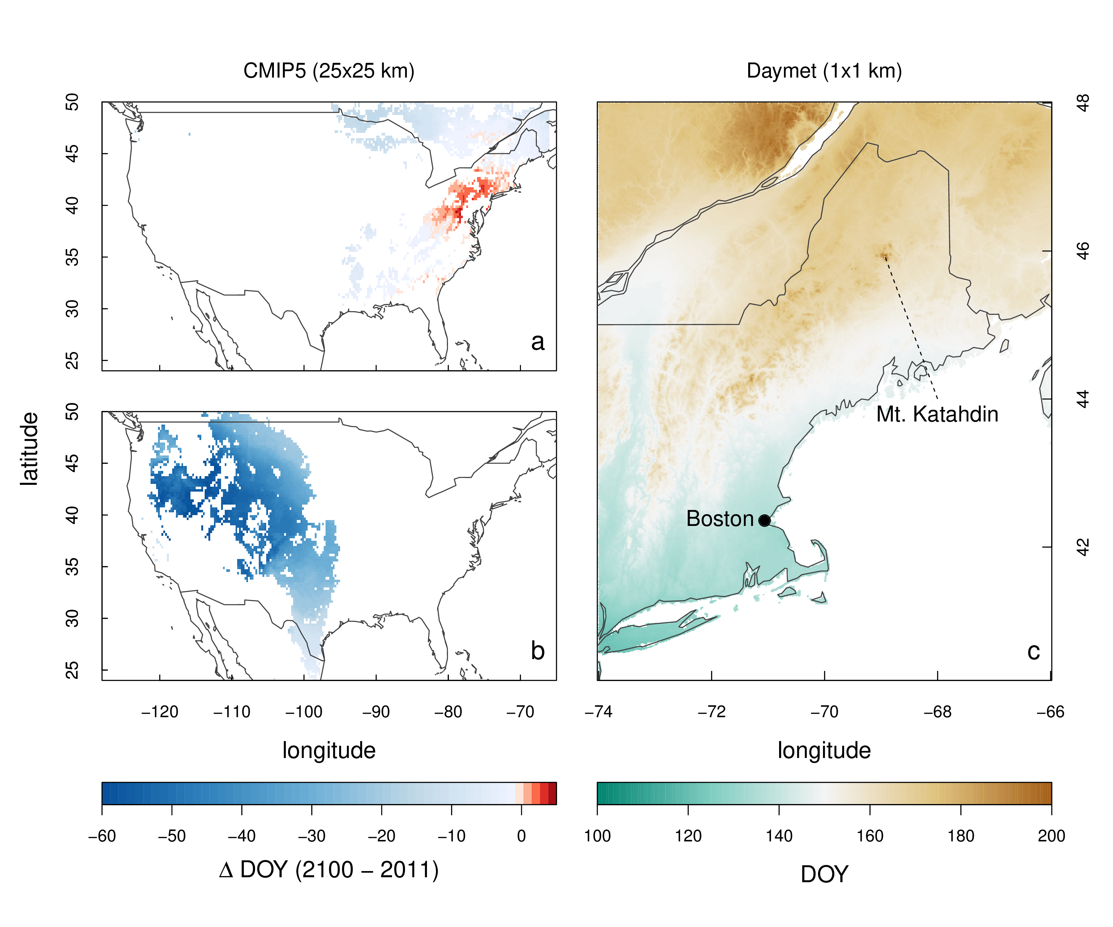 Overview map comparing various spatial outputs of the Thermal Time (TT) and Accumulated Growing Season Index (AGSI) model optimized to deciduous broadleaf and grassland PhenoCam data respectively. a) phenor model output of the difference in estimates of spring phenology between the year 2100 and 2011 for 1/4th degree NASA Earth Exchange (NEX) global gridded Coupled Model Intercomparison Project 5 (CMIP5) Mid-Resolution Institut Pierre Simon Laplace Climate Model 5 (IPSL-CM5A-MR) model runs using the TT model parameterized on deciduous forest PhenoCam sites. Only pixels with more than 50% deciduous broadleaf or mixed forest cover per 1/4th degree pixel, using MODIS MCD12Q1 land cover data, are shown; b) phenor model output of the difference in estimates of spring phenology between the year 2100 and 2011 for NEX CMIP5 IPSL-CM5A-MR model runs using the AGSI model parameterized on grassland PhenoCam sites. Only pixels with more than 50% grassland coverage per 1/4th degree pixel, using MODIS MCD12Q1 land cover data, are shown; c) phenor model output for 11 Daymet gridded datasets (tiles) for the year 2011.
References
Hufkens K., Basler J. D., Milliman T. Melaas E., Richardson A.D. 2018 An integrated phenology modelling framework in R: Phenology modelling with phenor. Methods in Ecology & Evolution, 9: 1-10.
Richardson, A.D., Hufkens, K., Milliman, T., Aubrecht, D.M., Chen, M., Gray, J.M., Johnston, M.R., Keenan, T.F., Klosterman, S.T., Kosmala, M., Melaas, E.K., Friedl, M.A., Frolking, S. 2018. Tracking vegetation phenology across diverse North American biomes using PhenoCam imagery. Scientific Data, 5, 180028.
Acknowledgements
This project was is supported by the National Science Foundation’s Macro-system Biology Program (awards EF-1065029 and EF-1702697) and the Marie Skłodowska-Curie Action (H2020 grant 797668). Logo design elements are taken from the FontAwesome library according to these terms.