![]()
![]()
![]()
A tool to calculate geolocation by light positions using sky illuminance values (in lux). The routine uses model optimization and parameter estimation to determine locations robustly.
How to cite this package
You can cite this package like this “we obtained location estimates using the {skytrackr} R package (Hufkens 2023)”. Here is the full bibliographic reference to include in your reference list (don’t forget to update the ‘last accessed’ date):
Hufkens, K. (2023). skytrackr: a sky illuminance location tracker. Zenodo. https://doi.org/10.5281/zenodo.8331492.
Installation
development release
To install the development releases of the package run the following commands:
if(!require(remotes)){install.packages("remotes")}
remotes::install_github("bluegreen-labs/skytrackr")
library("skytrackr")
Vignettes are not rendered by default, if you want to include additional documentation please use:
if(!require(remotes)){install.packages("remotes")}
remotes::install_github("bluegreen-labs/skytrackr", build_vignettes = TRUE)
library("skytrackr")
Use
To demonstrate the functioning of the package a small demo dataset comprised of a single day of light logging of a Common swift near a nest box in Ghent, Belgium was included (i.e. tag cc874). I will use this data to demonstrate the features of the package. Note that when multiple dates are present all dates will be considered. The package is friendly to the use of R piped (|>) commands. Using all default settings you can just pipe the data in to the skytrackr() function. The returned object will be a data frame containing the best estimate (median) of the longitude and latitude as well as 5-95% quantile as sampled from the posterior parameter distribution.
Data pre-screening
During the breeding season it is advised to remove data which is affected by time spent on a nest, altering the light signal and position estimates. Both the light patterns and other sensory data can be used to restrict the data to migration and non-breeding movements.
In the package I include the stk_profile() function which plots .lux files (and their ancillary .deg data) in an overview plot. The default plot is a static plot, however calling the function using the plotly = TRUE argument will render a dynamic plot on which you can zoom and which provides a tooltip showing the data values (including the date / time).
# read in the lux file, if a matching .deg
# file is found it is integrated into one
# long oriented data format
df <- stk_read_lux("your_lux_file.lux")

# plot the data using plotly show
stk_profile(df, plotly = TRUE)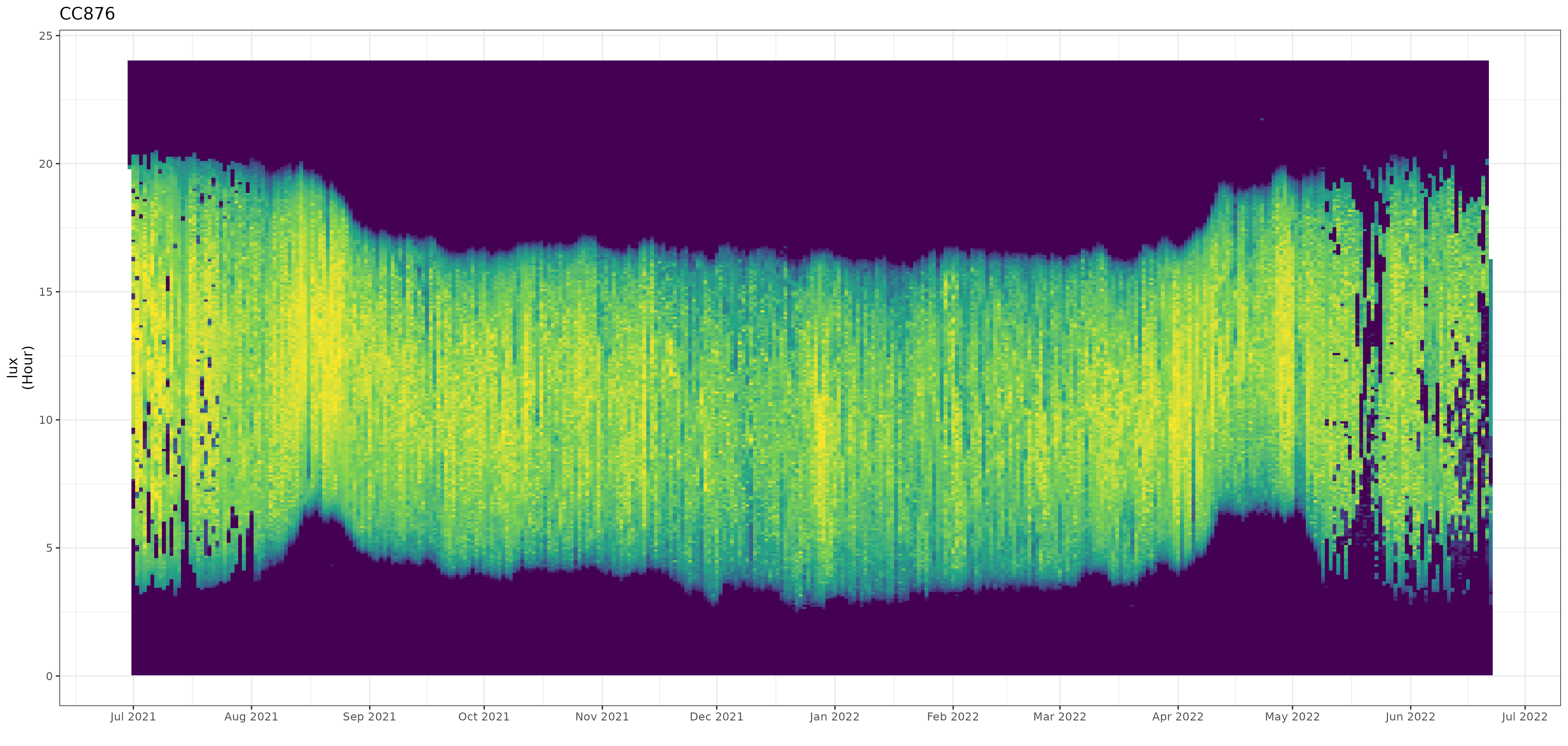
Date and time values of the non-breeding season can easily be determined and used in further sub-setting of the data for final processing.
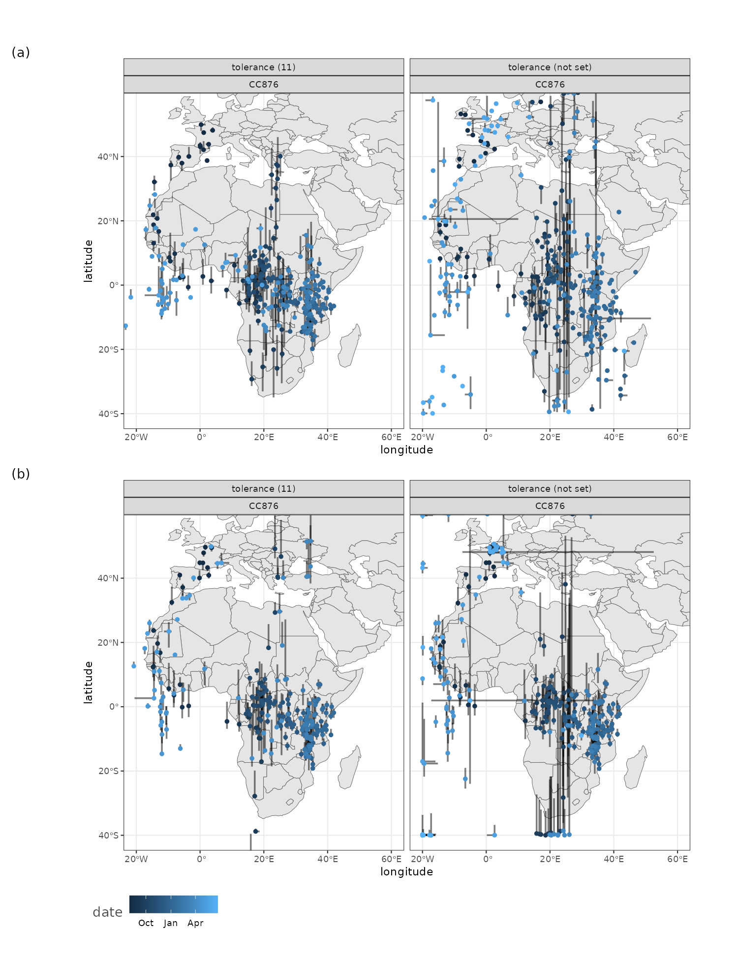
Default Sequential Monte Carlo optimization
The underlying BayesianTools package used in optimization allows for the specification of optimization techniques including Sequential Monte Carlo (SMC) method which is set as the default.This method is considerably faster than the MCMC DEzs method while fostering better accuracy during equinox periods, given a clean start position of the track. Note that care should be taken to specify the start location and tolerance (maximum degrees covered in a single flight). When results are unstable switch to DEzs optimization below.