Plot skytrackr results

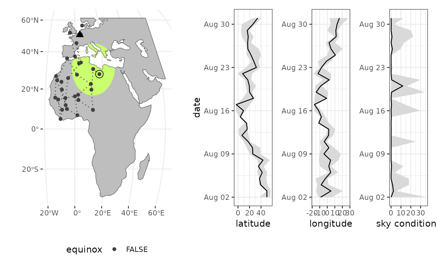
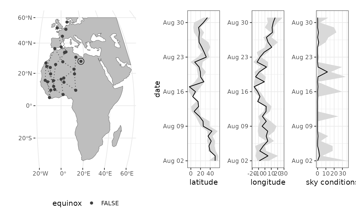
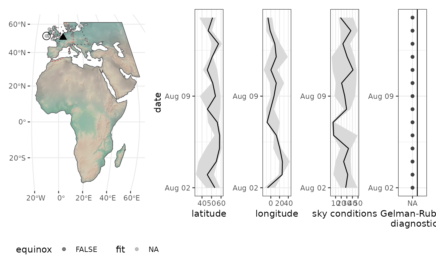
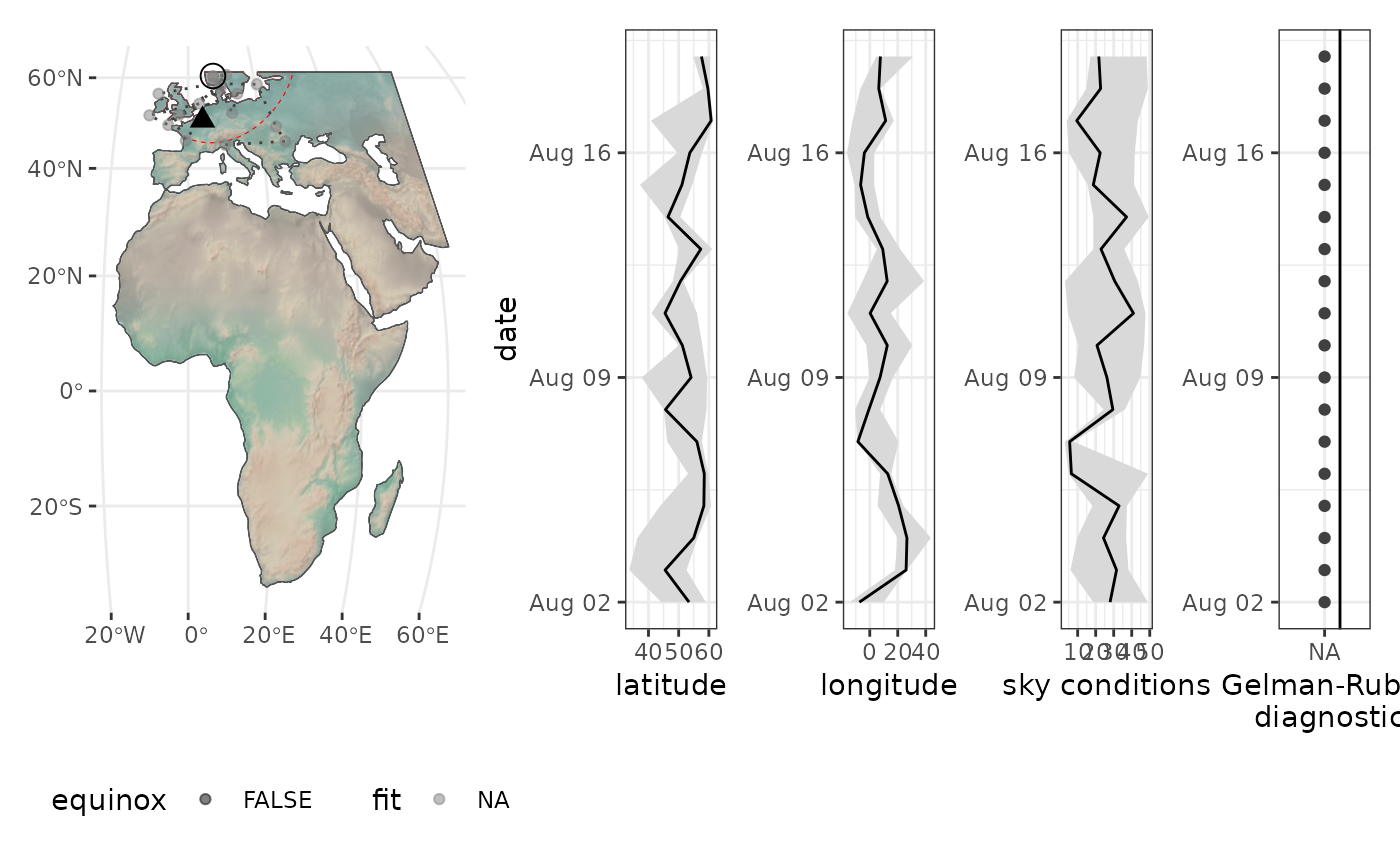
Create a map of estimated locations as a static or dynamic map.

stk_map(df, bbox, start_location, roi, dynamic = FALSE)

Arguments

df

A data frame with locations produced with the skytrackr() function

bbox

A geographic bounding box provided as a vector with the format xmin, ymin, xmax, ymax.

start_location

A start location as lat/lon to indicate the starting position of the track (optional)

roi

A region of interest under consideration, only used in plots during optimization

dynamic

Option to create a dynamic interactive graph rather than a static plot. Both the path as the locations are shown. The size of the points is proportional to the latitudinal uncertainty, while equinox windows are marked with red points. (default = FALSE)

Value

A ggplot map of tracked locations or mapview dynamic overview.

Examples

# \donttest{

# define land mask with a bounding box
# and an off-shore buffer (in km), in addition
# you can specify the resolution of the resulting raster
mask <- stk_mask(
  bbox  =  c(-20, -40, 60, 60), #xmin, ymin, xmax, ymax
  buffer = 150, # in km
  resolution = 0.5 # map grid in degrees
  )

  # define a step selection distribution/function
  ssf <- function(x, shape = 0.9, scale = 100, tolerance = 1500){
  norm <- sum(stats::dgamma(1:tolerance, shape = shape, scale = scale))
  prob <- stats::dgamma(x, shape = shape, scale = scale) / norm
}

# estimate locations
locations <- cc876 |> skytrackr(
  plot = TRUE,
  mask = mask,
  step_selection = ssf,
  start_location = c(50, 4),
      control = list(
        sampler = 'DEzs',
        settings = list(
        iterations = 10, # change iterations
         message = FALSE
        )
      )
  )
#> 
#> ══ Estimating locations ══════════════════════════════════════ skytrackr v1.1 ══
#> 
#> ℹ Processing logger: CC876!
#> 
#> ── Filtering data ──────────────────────────────────────────────────────────────
#> 
#> → Smoothing the data using a Hampel filter
#> ℹ Outliers will be replaced with interpolated values.
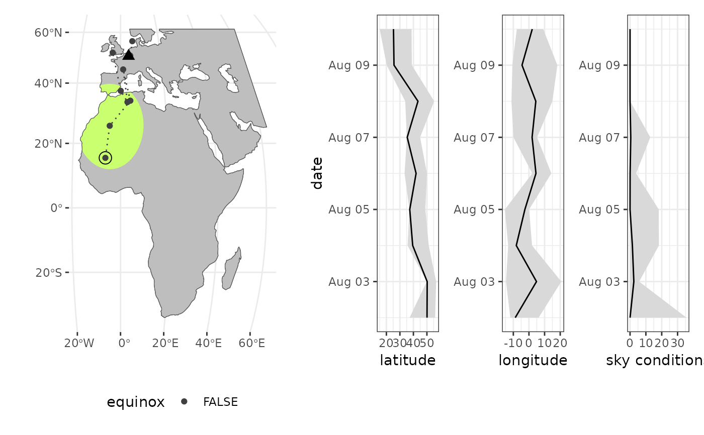
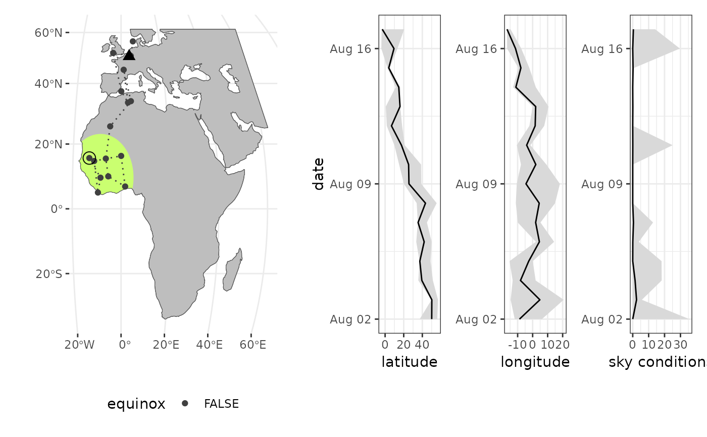
#> ℹ (preview plot will update every 2 days)

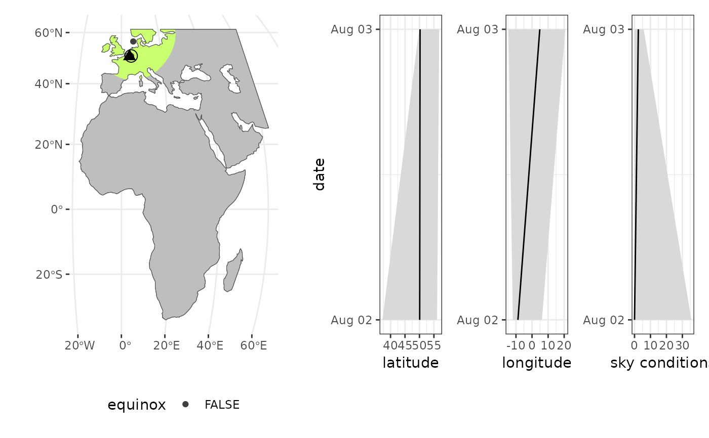#>  - Estimating positions ■■■■                              10% | ETA: 24s

#>  - Estimating positions ■■■■■■                            17% | ETA: 23s

#>  - Estimating positions ■■■■■■■■                          23% | ETA: 22s


#>  - Estimating positions ■■■■■■■■■■■■                      37% | ETA: 19s

#>  - Estimating positions ■■■■■■■■■■■■■■                    43% | ETA: 17s

#>  - Estimating positions ■■■■■■■■■■■■■■■■■                 53% | ETA: 14s


#>  - Estimating positions ■■■■■■■■■■■■■■■■■■■■              63% | ETA: 12s

#>  - Estimating positions ■■■■■■■■■■■■■■■■■■■■■■            70% | ETA: 10s

#>  - Estimating positions ■■■■■■■■■■■■■■■■■■■■■■■■          77% | ETA:  8s


#>  - Estimating positions ■■■■■■■■■■■■■■■■■■■■■■■■■■■■      90% | ETA:  3s

#>  - Estimating positions ■■■■■■■■■■■■■■■■■■■■■■■■■■■■■■    97% | ETA:  1s
#>  - Estimating positions ■■■■■■■■■■■■■■■■■■■■■■■■■■■■■■■  100% | ETA:  0s

#> ℹ Data processing done ...

#----- actual plotting routines ----
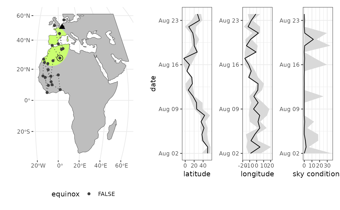
# static plot, with required bounding box
locations |> stk_map(bbox = c(-20, -40, 60, 60))


# dynamic plot
locations |> stk_map(dynamic = TRUE)
#> Warning: no non-missing arguments to min; returning Inf
#> Warning: no non-missing arguments to max; returning -Inf
# }