Model prediction

Koen Hufkens

2026-04-20

Once a model is calibrated you can use these parameters in a simulation, or when other known parametes are provided to you use those. Parameters are returned by the calibration routined as a nested list and should be provided as such to the prediction function hr_predict().

params <- list(
  r_l = 27.5332236990522,
  w_l = 0,
  r_d = 0.018257876686841,
  w_d = 0.9999,
  r_dist = 0.0412536435305482,
  w_dist = 0.9999,
  step_length_dist = 0.00216275705935606,
  step_length_shape = 1.14267311221975,
  threshold_approx_kernel = 7000,
  threshold_memory_kernel = 1000,

  # resource selection coefficients should be
  # a named list for driver data layer validation
  # and correct data processing
  coef = c(
    "slope" = 0.272835968106296,
    "slope_sq" = -0.093687792157105,
    "tcd_325grain"= 0.177991482087775,
    "tcd_325grain_sq" = -0.140639949444926,
    "landcover_5322" = 0.591063382485486,
    "landcover_agri" = -0.811974081226742
  )
)

Similar to the parameter fitting routine the function needs driver data and a set of parameters, as well as observations. Using the data used in the fitting routine and the above parameters (from Ranc et al. 2022) we can call hr_predict().

output <- hr_predict(
  data = drivers,
  par = params,
  obs = obs,
  runs = 2,
  steps = 20
)
#> Reading data table, run time: 64 ms
#> lookup tables, run time: 65 ms
#> Simulation mode
#> gros calculs, run time: 159 ms
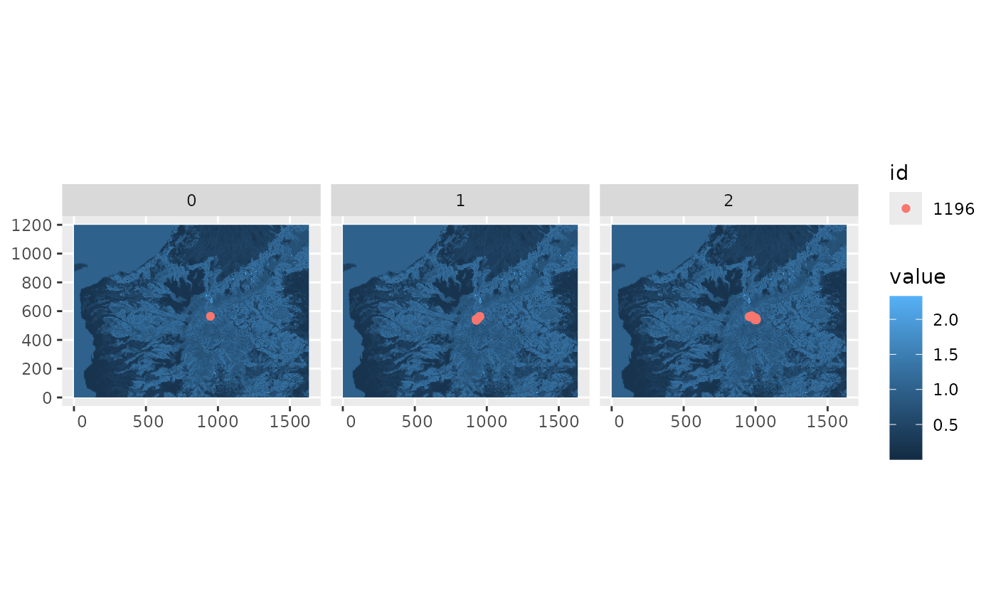
#> MODEL RUN ENDS, run time: 0 seconds

Simulations are generally fast so no parallel processing is provided. You can visualize the output by calling the plot() method.

plot(output)