hwsdr v2.0 functionality

Koen Hufkens

2024-02-04

Although the package provides support for the programmatic interface to the Harmonized World Soil Database ‘HWSD’ web services (https://daac.ornl.gov/cgi-bin/dsviewer.pl?ds_id=1247), a newer HWSD v2.0 version of the database has been released by the Food and Agriculture Organization (FAO). However, this version is not yet available on the ORNL DAAC. In the mean time, I provide point and region based extraction of data through the package with minimal manual downloads or data manipulations. In short, aside from the downloading of a single map (indices) the process largely remains similar to the use of the ORNL DAAC API.

Use

Download the base map

The HWSD v2.0 data is distributed as a spatial map where homogeneous regions are indicated with indices (integers). Although the underlying database is included in the package and can be accessed using hwsdr::hwsd2, the spatial data accompanying the database is too large for inclusion in the package. This spatial data needs to be downloaded explicitly.

Ideally, to speed up processing between sessions you download the data to a fixed location (directory) on your computer. The function ws_download() will download the data there. If successful the function will return the path where the data is located.

# set the ws_path variable using a FULL path name
path <- ws_download(
  ws_path = "/your/full/path",
  verbose = TRUE
)

To create persistence of the data between sessions, you can set the ~.Renviron file to contain a WS_PATH variable pointing to the directory where you downloaded the data. This environmental variable will then be read at startup and will be the default file location when using the hwsdr package for v2.0 data.

To set the .Renviron file you can use the usethis package and the usethis::edit_r_environ() function, which will create the file and open it in RStudio for you to edit.

usethis::edit_r_environ()

In the editor window you can then write:

WS_PATH = "/your/full/path"

A restart of the R(Studio) session is required for this to be considered in further processing. After this you can call the path by using Sys.getenv("WS_PATH") and passing the value to the ws_path parameter in ws_subset(). Al;ternatively you set it manually, and keep track of the gridded file location yourself in all your scripts.

Single pixel location download

Get world soil values for a single site using the following format, specifying coordinates as a pair of longitude, latitude coordinates (longitude, latitude). Here the call only extracts the top soil (layer = “D1”) fraction of sand and silt (% weight) for one specific location. Note that unlike HWSD v1.2 as available through the ORNL DAAC API the new version of the database has seven layers (D1 - D7) instead of just a top soil and sub-soil layer.

values <- ws_subset(
  site = "HWSD_V2",
  location = c(-81, 34),
  param = c("SAND","SILT"),
  layer = "D1",
  version = "2.0",
  ws_path = "/your/full/path"
)

At this location we have a top soil fraction of sand of 78% weight and a silt fraction of 12 % weight! Data are returned as tidy data frames including basic meta-data of the query for later subsetting.

print(values)
#> # A tibble: 2 × 5
#>   value latitude longitude site  parameter
#>   <dbl>    <dbl>     <dbl> <chr> <chr>    
#> 1    50       34       -81 HWSD  SAND     
#> 2    24       34       -81 HWSD  SILT

Gridded data

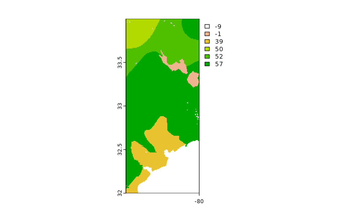
You can grab gridded data by specifying a bounding box c(lon, lat, lon, lat) defined by a bottom left and top right coordinates. Here the call only extracts the top soil (D1 layer) fraction of sand (%).

sand <- ws_subset(
    location = c(-81, 32, -80, 34),
    param = "SAND",
    layer = "D1",
    version = "2.0",
    ws_path = Sys.getenv("WS_PATH"),
    # ws_path = "/your/full/path",
    internal = TRUE
  )

terra::plot(sand)

Alternatively you can use sf bounding box (st_bbox()) function output to define an extent over which you want to extract gridded data. The structure of the function also allows for pipes to be used.

  a <- sf::st_sf(a = 1:2,
                geom = sf::st_sfc(
                  sf::st_point(c(34, -81)),
                  sf::st_point(c(32, -80))),
                crs = 4326)

  t_sand <- a %>%
    sf::st_bbox() %>%
    ws_subset(
      version = "2.0",
      param = "SAND",
      layer = "D1",
      ws_path = Sys.getenv("WS_PATH")
      )

This call gives an equivalent dataset as above, as shown in the plot.

terra::plot(sand)