skylight advanced
Koen Hufkens
2026-01-11
Source:vignettes/skylight_advanced.Rmd
skylight_advanced.RmdCloud cover correction
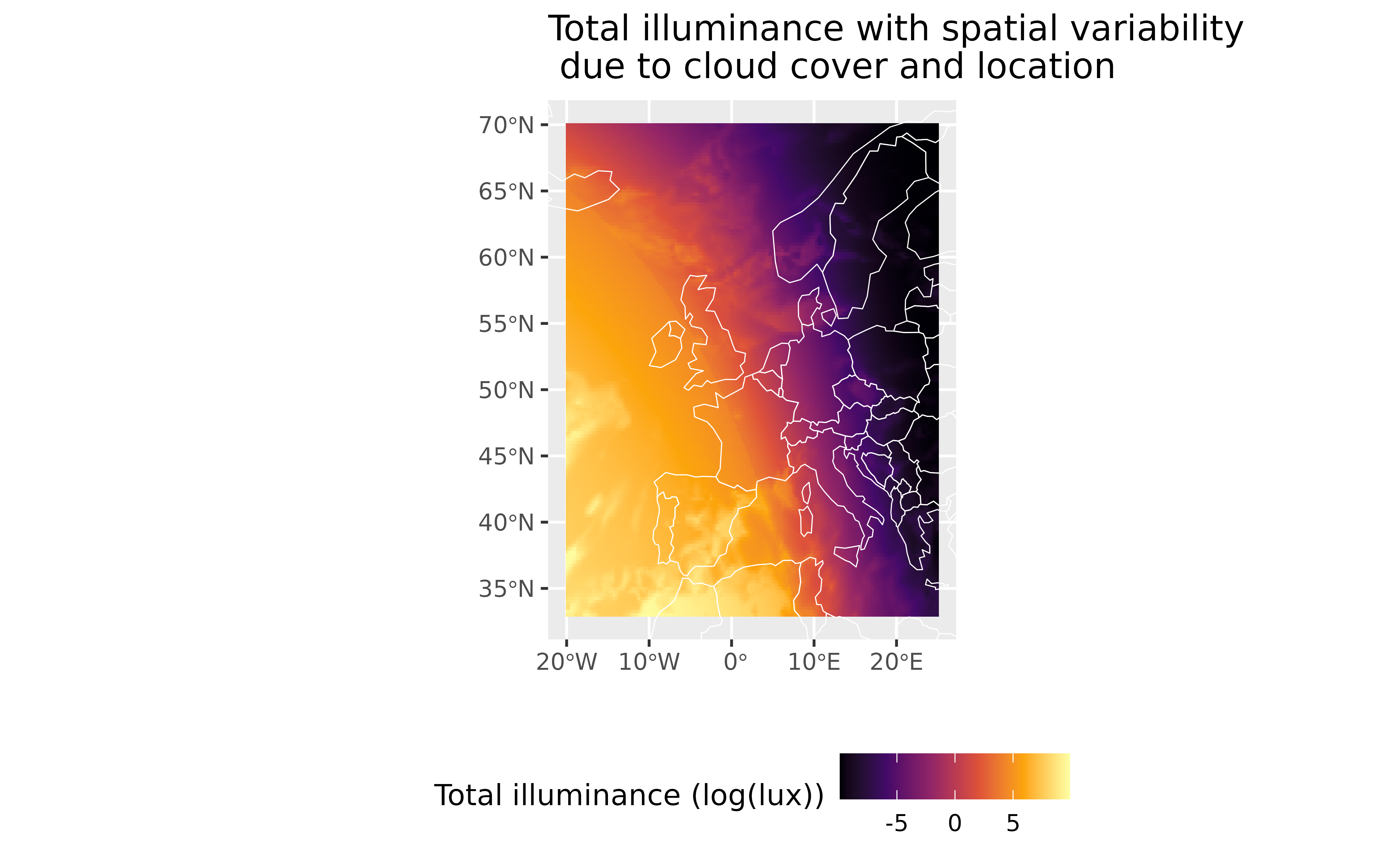
The original implementation of the software allows for a correction of illuminance based upon three cloud cover conditions. However, this is in all practical sense a simple scaling of the data (see Janiczek and DeYoung 1987). You can either apply this scaling factor, a division by a number greater than 1 using the function itself, or apply it post-hoc on the returned values. Below I show an example routine to use the internal scaling, using ERA5 total cloud cover (tcc) data.
Downloading cloud cover data
To provide our analysis with cloud cover data I rely on the BlueGreen
Labs ecmwfr
package. So, I first query some total cloud cover data (0 - 1) covering
most of Europe.
library(ecmwfr)

request <- list(
  product_type = "reanalysis",
  format = "netcdf",
  variable = "total_cloud_cover",
  year = "2021",
  month = "02",
  day = "01",
  time = c("00:00", "01:00", "02:00", "03:00", "04:00",
           "05:00", "06:00", "07:00", "08:00", "09:00",
           "10:00", "11:00", "12:00", "13:00", "14:00",
           "15:00", "16:00", "17:00", "18:00", "19:00",
           "20:00", "21:00", "22:00", "23:00"),
  area = c(70, -20, 33, 25),
  dataset_short_name = "reanalysis-era5-single-levels",
  target = "era5.nc"
)

wf_request(
  user = "xxxx",
  request = request,
  transfer = TRUE
)
Downloaded data can be read with the terra package. The
above downloaded data is included as a demo data set in the package. You
can therefore use this included data in this workflow. Check out the
ecmwfr package to download your own custom data.
#> terra 1.8.86
library(terra)

# read in data
era5 <- terra::rast(system.file(package = "skylight", "extdata/era5.nc"))

# use this command when downloading the data yourself
# era5 <- terra:rast(file.path(tempdir(),"era5.nc"))
However, the spatial format needs to be converted to a data frame for
use with the skylight package.
library(dplyr)
#>
#> Attaching package: 'dplyr'
#> The following objects are masked from 'package:terra':
#>
#>     intersect, union
#> The following objects are masked from 'package:stats':
#>
#>     filter, lag
#> The following objects are masked from 'package:base':
#>
#>     intersect, setdiff, setequal, union

# create a data frame with values
df <- era5 |>
  as.data.frame(xy = TRUE) |>
  rename(
    longitude = "x",
    latitude = "y"
  )

# add the original time stamp
df$date <- time(era5)

print(head(df))
#>   longitude latitude       tcc                date
#> 1    -20.00       70 0.9886775 2021-02-01 17:00:00
#> 2    -19.75       70 0.9975280 2021-02-01 17:00:00
#> 3    -19.50       70 0.9941709 2021-02-01 17:00:00
#> 4    -19.25       70 0.9639876 2021-02-01 17:00:00
#> 5    -19.00       70 0.9417698 2021-02-01 17:00:00
#> 6    -18.75       70 0.9416477 2021-02-01 17:00:00
library(skylight)

# calculate sky illuminance values for
# a single date/time and location
df <- df |>
  mutate(
    # values of cloud cover lower than
    # 30% are considered clear conditions
    # for the skylight model - adjust tcc values
    tcc = ifelse(tcc <= 0.3, 1, tcc),
    # rescale total cloud cover between 1 - 10
    # the acceptable range for skylight's
    # sky_condition parameter
    sky_condition = scales::rescale(df$tcc, to = c(1,10))
  )

# pipe into skylight
df <- df |> skylight()

print(head(df))
#>   longitude latitude       tcc                date sky_condition sun_azimuth
#> 1    -20.00       70 0.9886775 2021-02-01 17:00:00      9.898097         229
#> 2    -19.75       70 0.9975280 2021-02-01 17:00:00      9.977752         229
#> 3    -19.50       70 0.9941709 2021-02-01 17:00:00      9.947538         229
#> 4    -19.25       70 0.9639876 2021-02-01 17:00:00      9.675888         229
#> 5    -19.00       70 0.9417698 2021-02-01 17:00:00      9.475928         230
#> 6    -18.75       70 0.9416477 2021-02-01 17:00:00      9.474829         230
#>   sun_altitude sun_illuminance moon_azimuth moon_altitude moon_illuminance
#> 1    -3.983115        2.511910            2     -17.60419     5.917033e-13
#> 2    -4.047531        2.332974            3     -17.60053     5.892869e-13
#> 3    -4.112172        2.190011            3     -17.59649     5.936460e-13
#> 4    -4.177039        2.106323            3     -17.59205     6.132194e-13
#> 5    -4.242130        2.011334            3     -17.58723     6.294024e-13
#> 6    -4.307443        1.880456            4     -17.58203     6.329976e-13
#>   moon_fraction total_illuminance
#> 1      81.93127          2.511960
#> 2      81.93127          2.333024
#> 3      81.93127          2.190061
#> 4      81.93127          2.106374
#> 5      81.93127          2.011387
#> 6      81.93127          1.880509
I can now plot the sky illuminance as corrected for cloud cover using the internal scaling factor. Keep in mind that this is a rather ad-hoc solution. For proper results external empirical relationships should be established between the model response and measured illuminance values under varying cloud cover conditions.
library(ggplot2)
library(rnaturalearth)

# country outlines
outlines <- rnaturalearth::ne_countries(returnclass = "sf")

ggplot(df) +
  geom_tile(
    aes(
      longitude,
      latitude,
      fill = log(total_illuminance)
    )
  ) +
  scale_fill_viridis_c(
    option = "B",
    name = "Total illuminance (log(lux))"
  ) +
  geom_sf(
    data = outlines,
    colour = "white",
    fill = NA
    ) +
  coord_sf(
    xlim = c(-20, 25),
    ylim = c(33, 70)
  ) +
  labs(
    title = "Total illuminance with spatial variability\n due to cloud cover and location",
    y = "",
    x = ""
  ) +
  theme(
    legend.position = "bottom"
  )

