snotelr functionality
Koen Hufkens
2026-01-11
Source:vignettes/snotelr-vignette.Rmd
snotelr-vignette.RmdIntroduction
The SNOTEL network is composed of over 800 automated data collection sites located in remote, high-elevation mountain watersheds in the western U.S. They are used to monitor snowpack, precipitation, temperature, and other climatic conditions. The data collected at SNOTEL sites are transmitted to a central database. This package queries this centralized database to provide easy access to these data and additional seasonal metrics of snow accumulation (snow phenology).
Downloading site meta-data
The SNOTEL network consists of a vast number of observation sites,
all of them listed together with their meta-data on the SNOTEL website.
The snotel_info() function allows you to query this table
and import it as a neat table into R. Some of the
meta-data, in particular the site id (site_id), you will
need of you want to download the data for a site. You can save this
table to disk using the path variable to specify a location
on your computer where to store the data as a csv. If this parameter is
missing the data is returned as an R variable.
# download and list site information
site_meta_data <- snotel_info()
head(site_meta_data)
#>   network state            site_name
#> 1    SNTL    AK     elmendorf field
#> 2    SNTL    CO          alta lakes
#> 3    SNTL    MT          mill creek
#> 4    SNTL    UT           elk ridge
#> 5    SNTL    AK              hoonah
#> 6    SNTL    AK pilgrim hot springs
#>                                    description      start        end latitude
#> 1             Outlet Ship Creek (190204010404) 2024-10-01 2026-01-11    61.25
#> 2   South Fork San Miguel River (140300030103) 2025-09-01 2026-01-11    37.89
#> 3              Upper Mill Creek (100700020302) 2025-07-01 2026-01-11    45.26
#> 4              Cottonwood Creek (140802010402) 2024-10-01 2026-01-11    37.82
#> 5                 Port Fredrick (190102110906) 2023-10-01 2026-01-11    58.12
#> 6 Paystreak Creek-Pilgrim River (190501050702) 2024-07-01 2026-01-11    65.09
#>   longitude elev        county site_id
#> 1   -149.82   52     Anchorage    1332
#> 2   -107.84 3441    San Miguel    1344
#> 3   -110.41 2262          Park    1322
#> 4   -109.77 2603      San Juan    1323
#> 5   -135.41  463 Hoonah-angoon    1318
#> 6   -164.92    6          Nome    1327
Downloading site data
If you downloaded the meta-data for all sites you can make a
selection using either geographic coordinates, or state
columns. For the sake of brevity I’ll only query data for one site using
its site_id below. By default the data, reported in
imperial values, are converted to metric measurements.
# downloading data for a random site
snow_data <- snotel_download(
  site_id = 670,
  internal = TRUE
  )
#> Downloading site: northeast entrance , with id: 670

# show the data
head(snow_data)
#>   network state           site_name                           description
#> 1    SNTL    MT northeast entrance  Upper Soda Butte Creek (100700010602)
#> 2    SNTL    MT northeast entrance  Upper Soda Butte Creek (100700010602)
#> 3    SNTL    MT northeast entrance  Upper Soda Butte Creek (100700010602)
#> 4    SNTL    MT northeast entrance  Upper Soda Butte Creek (100700010602)
#> 5    SNTL    MT northeast entrance  Upper Soda Butte Creek (100700010602)
#> 6    SNTL    MT northeast entrance  Upper Soda Butte Creek (100700010602)
#>        start        end latitude longitude elev county site_id       date
#> 1 1937-10-01 2026-01-11    45.01   -110.01 2262   Park     670 1966-10-01
#> 2 1937-10-01 2026-01-11    45.01   -110.01 2262   Park     670 1966-10-02
#> 3 1937-10-01 2026-01-11    45.01   -110.01 2262   Park     670 1966-10-03
#> 4 1937-10-01 2026-01-11    45.01   -110.01 2262   Park     670 1966-10-04
#> 5 1937-10-01 2026-01-11    45.01   -110.01 2262   Park     670 1966-10-05
#> 6 1937-10-01 2026-01-11    45.01   -110.01 2262   Park     670 1966-10-06
#>   snow_water_equivalent snow_depth precipitation_cumulative temperature_max
#> 1                   0.0         NA                       NA              NA
#> 2                   7.6         NA                       NA              NA
#> 3                   0.0         NA                       NA              NA
#> 4                   0.0         NA                       NA              NA
#> 5                   0.0         NA                       NA              NA
#> 6                   0.0         NA                       NA              NA
#>   temperature_min temperature_mean precipitation
#> 1              NA               NA            NA
#> 2              NA               NA            NA
#> 3              NA               NA            NA
#> 4              NA               NA            NA
#> 5              NA               NA            NA
#> 6              NA               NA            NA
# A plot of snow accummulation through the years
plot(as.Date(snow_data$date),
     snow_data$snow_water_equivalent,
     type = "l",
     xlab = "Date",
     ylab = "SWE (mm)"
    )
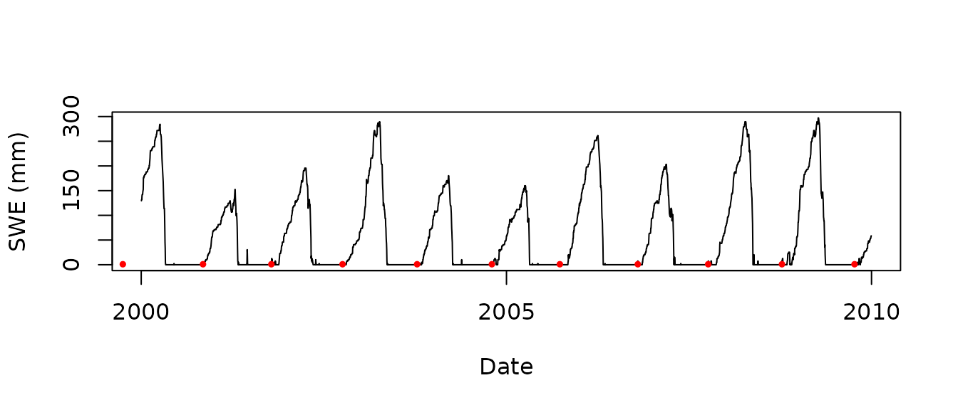
Calculating snow phenology from downloaded data or data frames
Although the main function of the package is to provide easy access
to the SNOTEL data a function snotel_phenology() is
provided to calculate seasonal metrics of snow deposition.
# calculate snow phenology
phenology <- snotel_phenology(snow_data)
#> Joining with `by = join_by(date)`
# subset data to the first decade of the century
snow_data_subset <- subset(snow_data, as.Date(date) > as.Date("2000-01-01") &
                             as.Date(date) < as.Date("2010-01-01"))

# plot the snow water equivalent time series
plot(as.Date(snow_data_subset$date),
     snow_data_subset$snow_water_equivalent,
     type = "l",
     xlab = "Date",
     ylab = "SWE (mm)"
  )

# plot the dates of first snow accumulation as a red dot
points(phenology$first_snow_acc,
       rep(1,nrow(phenology)),
       col = "red",
       pch = 19,
       cex = 0.5
      )
A list of all provided snow phenology statistics is provided below.
| Value | Description |
|---|---|
| year | The year in which the an event happened |
| first_snow_melt | day of first full snow melt (in DOY) |
| cont_snow_acc | start of continuous snow accumulation / retention (in DOY) |
| last_snow_melt | day on which all snow melts for the remaining year (in DOY) |
| first_snow_acc | day on which the first snow accumulates (in DOY) |
| max_swe | maximum snow water equivalent value during a given year (in mm) |
| max_swe_doy | day on which the maximum snow water equivalent value is reached (in DOY) |