The skytrackr R package
a template matching approach to geolocation by light
Koen Hufkens
Source:vignettes/skytrackr_vignette.Rmd
skytrackr_vignette.Rmd1 Abstract
The {skytrackr} R package provides a convenient template fitting methodology (Ekstrom 2004) and a Bayesian based optimization approach to estimate geolocations from light. The use of additional data during twilight, or a full day, allows for automation of the process over threshold based methods. Including more data in location estimates, based upon a physical models of behaviour (step-selection), the physical light environment and additional parameters (such as a land mask) improve accuracy and reproducibility at a low labour cost, while also providing uncertainty measures for post-hoc quality control.
Keywords: geolocation, tracking, movement ecology, flight, illuminance
2 Background
Geolocation by light has been a popular animal tracking method in ornithology. It has been successfully used to track long distance migration and foraging behaviour of swifts Hedenström et al. (2019) and other migratory birds, and increased our understanding of these long-distance movements.
Geolocation by light is a conceptually easy approach. It relies mostly on the shift of sunrise and sunset times to determine longitude and the length of night (or day) between sunrise or sunset to determine latitude deterministically using astronomical equations (Ekstrom 2004). Two approaches are commonly used, firstly the twilight method, and secondly a template matching method.
In the twilight method considerable uncertainty is introduced due to the choice of the threshold in light levels used in determining sunset or sunrise times Joo et al. (2020). The choice of a proper threshold and solar angle is critical as it determines the day length and therefore estimates of latitude. As such, “Increasing mismatch between light intensity threshold and sun elevation threshold results in a decreasing accuracy in latitudinal estimation” (Lisovski and Hahn 2012). Given an unknown starting position and a reference day length to calibrate a threshold on this threshold is often estimated by eye. Alternatively, the template matching method leverages the full twilight transition profile to estimate locations (Ekstrom 2004). Although mostly sidestepping issues of picking threshold values, calibrations are still needed for the template matching method.
Ongoing research therefore often focuses on the use of ancillary data (e.g. air pressure data (Nussbaumer et al. 2023)) or computational methods to improve both the accuracy of estimates as well as the workflows involved. For example iterative methods can constrain the search space of optimal solutions better (Merkel et al. 2016). Twilight free methods have been explored by Bindoff et al. (2018) which uses a hidden markov model approach to constrain parameters using the full light level data and not explicitly sunrise and sunset thresholding. Despite these advances in methodology few computational resources are available to estimate positions in bulk with minimal intervention consistently.
Here, I present the {skytrackr} R package which provides a Bayesian optimization based approach using a physical sky illuminance model Janiczek and DeYoung (1987) to estimate geolocation from light levels. This package aims to provide a hands-off, explicit calibration free, robust methodology to automated (reproducible) geolocation estimates. The package uses both a physical and behavioural components (step-selection function) to constrain location estimates.
3 Implementation
3.1 Optimization strategy
The {skytrackr} R package uses a physical sky illuminance model Janiczek and DeYoung (1987) in combination with Bayesian location parameter estimation (Hartig et al. 2023) approach to maximise the log-likelihood between observed (logger) and modelled values combined with those of a step-selection model describing the animal’s behaviour.
Model parameters are limited to latitude, longitude and a sky condition, which scales the sky illuminance response for the day and is a free calibration parameter which is optimized together with the location parameters. The approach improves upon the template matching as suggested by Ekstrom (2004) by including a physical component to the model rather than considering a simpler piece-wise regression based approach, or more basic physical models. Below (Figure 3.1), is an example of how changes to both longitude or latitude influence the shape of the diurnal light profile. A change in longitude shifts the diurnal curve left to right (blue line), while a latitudinal change will influence the steepness and width of the curve (green line). An optimal fit (but not accounting for attenuation by clouds or a covered sensor) is shown as the red curve. The optimization routine tries to find the optimal fit (red line) using a combination of the above mentioned parameters (latitude, longitude, sky conditions) [while taking into account the probability of a step from the previously estimated location].
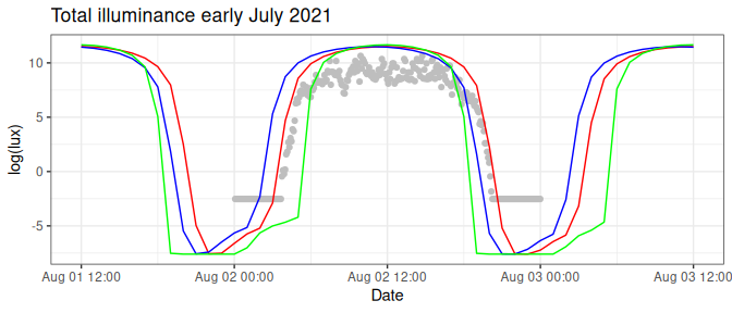
Figure 3.1: Modelled and observed illuminance values in log(lux) for three days in early July 2021. Observed values are shown as light grey dots, modelled values for the exact location are shown as a full red line. Longitudinal offset data is shown as the blue full line, while latitudinal offset modelled data for the same period is shown as a full green line.
By default, the DEzs MCMC sampler (Ter Braak and Vrugt 2008) implemented in BayesianTools (Hartig et al. 2023) is used to estimate the posterior distribution of model parameters. For each location I sample the posterior distribution of the parameters (with a thinning factor of 10), and return summary values. I return the maxiumum aposteriori values as the best estimate of latitude, longitude and sky conditions. In addition, the 5, 50, and 95% quantiles on the parameter distributions are provided. The package also returns the Gelman-Rubin-Brooks (GRB) metric (Gelman and Rubin 1992), which can be used to assess the convergence of the optimization. Both the quantile ranges and the GRB metric can be used in post-hoc quality control screening.
3.2 Behavioural component
In order to constrain location estimates, especially during equinoxes, behavioural prior knowledge is included during parameter optimization in the form of a step selection function from a previously estimated location. A step-selection function attributes a likelihood to the distance of every step and often takes the form of a gamma or Weibull function (Figure 3.2). The combined log-likelihood of both the parameter estimates of the physical model as well as the behavioural component are taken into account to optimize the final location estimate.
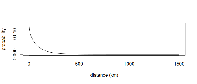
Figure 3.2: A step selection function showing the probability of moving a given distance from the previous location.
3.3 Workflow
The package workflow is aimed to be pipe (|>) friendly with data formats adhering to tidy data standards. The workflow is meant to be as hands off as possible, with sensible defaults.
3.3.1 Reading data
Two functions are provided to read common data formats, the Migrate Technology Ltd .lux and the Swiss Ornithological Institute (SOI) .glf data formats using stk_read_lux() and stk_read_glf() respectively. A small example dataset (.lux) is included to experiment with some of the package functionality.
# read in the lux file
df <- stk_read_lux(
      system.file("extdata/cc876.lux", package="skytrackr")
    )
#>
#> ══ Reading data ══════════════════════════════════════════════ skytrackr v2.0 ══
#>
#> ℹ Processing file: cc876.lux !
#>
#> ── Header information ──
#>
#>     “Migrate Technology Ltd logger Type: 13.2061.8, current settings:
#>     Approx 1'C resolution. Altimeter fitted. Light range 5, clipped
#>     OFF, max light regime, floor 0.08lux. Logger number: CC876
#>
#>     MODE: 15 (light, temperature, pressure recorded) LIGHT: Sampled
#>     every minute with max light recorded every 5mins. TEMPERATURE and
#>     PRESSURE: Sampled and recorded every 30mins. WET/DRY and
#>     CONDUCTIVITY: NOT RECORDED Max record length = 16 months. Total
#>     battery life approx 13 months. Logger is currently 13 months old.
#>
#>     Programmed: 29/06/2021 19:44:10. Start of logging (DD/MM/YYYY
#>     HH:MM:SS): 30/06/2021 19:44:10 Age at start of logging (secs):
#>     3923996, approx 2 months End of logging (DD/MM/YYYY HH:MM:SS):
#>     22/06/2022 16:15:21 Age at end of logging (secs): 34756240,
#>     approx 13 months Timer (DDDDD:HH:MM:SS): 00356:20:30:44 Drift
#>     (secs): 27. Memory not full.  Pointers:
#>     60380,209592,12105912,12105912,0,0,49,60% light mem used,68%
#>     wet/dry/temp mem used Tcals (Ax^3+Bx^2+Cx+D): NaN,NaN,NaN,NaN
#>     Approx 1'C resolution. Altimeter fitted. Light range 5, clipped
#>     OFF, max light regime, floor 0.08lux.”
#>     —
#>

# plot the data as a static plot
df |> stk_profile()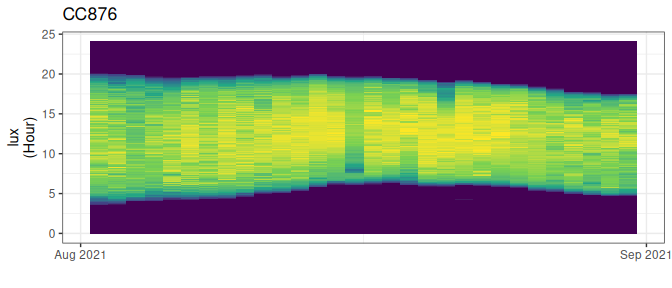
Figure 3.3: Light profile of a data logger
3.3.2 Cleaning data
Light logger data can be influenced by factors which make it impossible to correctly estimate location parameters. For example when no light is recorded when an animal is in a nest during twilight hours. To deal with these “false twilights” or spuriously low values during daytime a screening function is implemented to remove such days, only retaining those days with a reasonably complete diurnal light profile.
# introduce a false twilight
# by setting some twilight values very low
df <- df |>
  mutate(
    value = ifelse(
      date_time > "2021-08-15 05:00:00" & date_time < "2021-08-15 12:00:00",
      0.1,
      value)
  )

# plot false twilight
df |> stk_profile()
Figure 3.4: Data with a false twilight
You can then clean the data using stk_screen_twl(). If the argument filter is set to TRUE the offending day will be removed and not processed.
# screen for twilight and other disturbing factors
df <- df |> stk_screen_twl(filter = TRUE)

# plot the updated dataset
df |> stk_profile()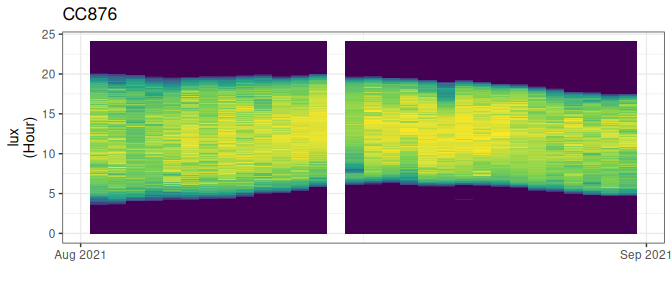
Figure 3.5: Screened light values, with offending days removed
Manual selection of regions of the light profile which are of good quality can also be used. A helpful tool in this context is the use of the interactive plotting using the plotly option of the stk_profile() function. This plotting option will allow you to inspect the light profiles with a tooltip to determine exact dates between which you would want to process data.
# visualize interactively
df |> stk_profile(plotly = TRUE)

# subset to a particular date range
df <- df |>
   filter(
   date >= "2019-08-31" & date <= "2020-04-15"
   )
3.3.3 Creating a land mask
The optimization routine relies on a land mask to constrain land based animals to land. This mask needs to be generated beforehand. The mask will generate a raster file showing land locations, buffered by a given distance (in km) and with a given spatial resolution (in degrees). Only locations within the mask are considered during location estimates. Should an animal not be constrained to land a mask (map) should be generated with unity (1) values throughout.
# generate a mask
mask <- stk_mask(
  bbox  =  c(-20, -40, 60, 60), #xmin, ymin, xmax, ymax
  buffer = 150, # in km
  resolution = 0.5
)

# plot the mask
plot(mask)
knitr::include_graphics("mask.png")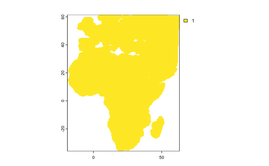
Figure 3.6: Land mask to constrain location estimates
3.3.4 Defining a step-selection
The location estimates are not only constrained by geography but more importantly by behaviour. A function (returning probabilities) can be used to weight the probability of a step of a particular distance (relative to the previous location). Although any function can be used common step-selection probability distributions such as a gamma or Weibull are adviced.
Here I do not recommend using a biophysical basis, based on flight speed or power functions, such as used in the {GeoPressureR} package. First, the flight distances are not a reflection of flight speed, as this depends on behaviour. In particular, local ranging at high speed might not result in large distances traveled as measured on a daily time step (the resolution of the analysis). Second, although migration is often the focus of bio-logging the bulk of the behaviour during any trip will not be spent migrating. In short, the step-selection function should reflect the most common local ranging behaviour at a daily time step in order to provide valid constraints during optimization. If available, previous data gathered and expert knowledge can be used to inform you on the shape of this step-selection function. Here, I’ll use a normalized gamma distribution as specified above and shown in Figure 3.2.
3.4 Estimating positions
After reading in the data, cleaning the data, and setting up the mask and step-selection function you can now call the main skytrackr() function. This function deals with the final parameter optimization (location estimates). Before proceeding you will have to set a few more parameters. In particular, a start location (which should be the location where you tagged your individual), the tolerance distance (in km) which sets a hard limit on the locations considered (redundant dependent on the shape of the step-selection function), the scale parameter which adjusts the daylight levels to occlusions by clouds (or fur/feathers/other environmental factors), the range of light values (in lux) to consider (to select either only twilight periods or the full diurnal cycle). Finally, you have to specify the control parameters for the BayesianTools functions as a nested list.
# set a random seed
# for reproducibility reasons
set.seed(1)

# estimate locations
locations <- df |>
    skytrackr(
      start_location = c(51.08, 3.73),
      tolerance = 1500,
      scale = log(c(0.00001,50)), # defaults
      range = c(0.09, 140), # defaults
      control = list(
        sampler = 'DEzs',
        settings = list(
          burnin = 250, # default
          iterations = 3000, # default
          message = FALSE
        )
      ),
      step_selection = ssf,
      mask = mask,
      plot = TRUE
    )
══ Estimating locations ══════════════════════════════════════ skytrackr v1.0 ══
ℹ Processing logger: CC876!
ℹ (preview plot will update every 7 days)
estimating positions ■■ 2% | ETA: 2hIf the plot parameter is set to TRUE a plot of the estimated locations will be generated every so many days (see parameter settings). For reference, processing a full year of data with the above settings takes approximately one hour, slightly faster without the preview plots. The red dashed outline highlights the search area for the best location estimate. The last estimated location is highlighted with an open circle.
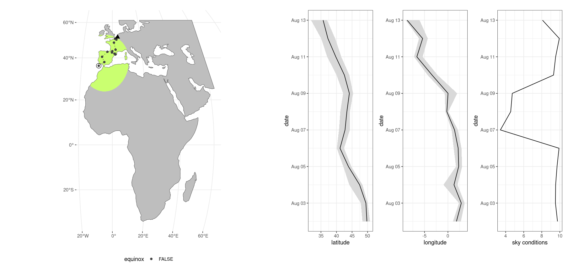
Figure 3.7: Dynamic preview during location estimation
3.4.1 Optimization caveats (advanced control settings)
Generally speaking around 3000 iterations, with 500 for burnin, should be sufficient to get reasonable parameter estimates. Using lower values can speed up the processing but at the cost of precision. The latter is important as there is a co-dependency between the current and the previous step through the distance based step-selection function. Hence, errors can propagate through auto-correlation. Increasing iterations has its limit, as 1500x1500 km (or ~150x150 degree, assuming a one degree search grid) search area could be efficiently searched using brute force with ~22K iterations. The use of an optimization based method is to avoid using expensive brute-force methods which impose overhead and quantization of the location estimates.
The default scale parameter range covers values from close to 0 to 50, far outside the normal range of the {skylight} sky illuminance model (with values normally ranging from 1 to 10). This larger range accounts for either the non-physical basis of the sensor and occlusions of the sensor decreasing light input (i.e. mediating the raw sensor response). This parameter should be set wide enough to allow for sufficient model flexibility, but not too wide as to inflate the parameter space to search (deteriorating parameter/location estimates through insufficient sampling coverage). You can get a reasonable estimate of the scale range by using the stk_calibrate() function.
Note: the final location estimates include all model settings as an output, too. This ensures that given the correct {skytrackr} version you can reproduce your results.
3.5 Visualizing location estimates
Running the full dataset for logger CC876, from which a subset is included, would yield a full track. You can visualize a full track using the stk_map() function.
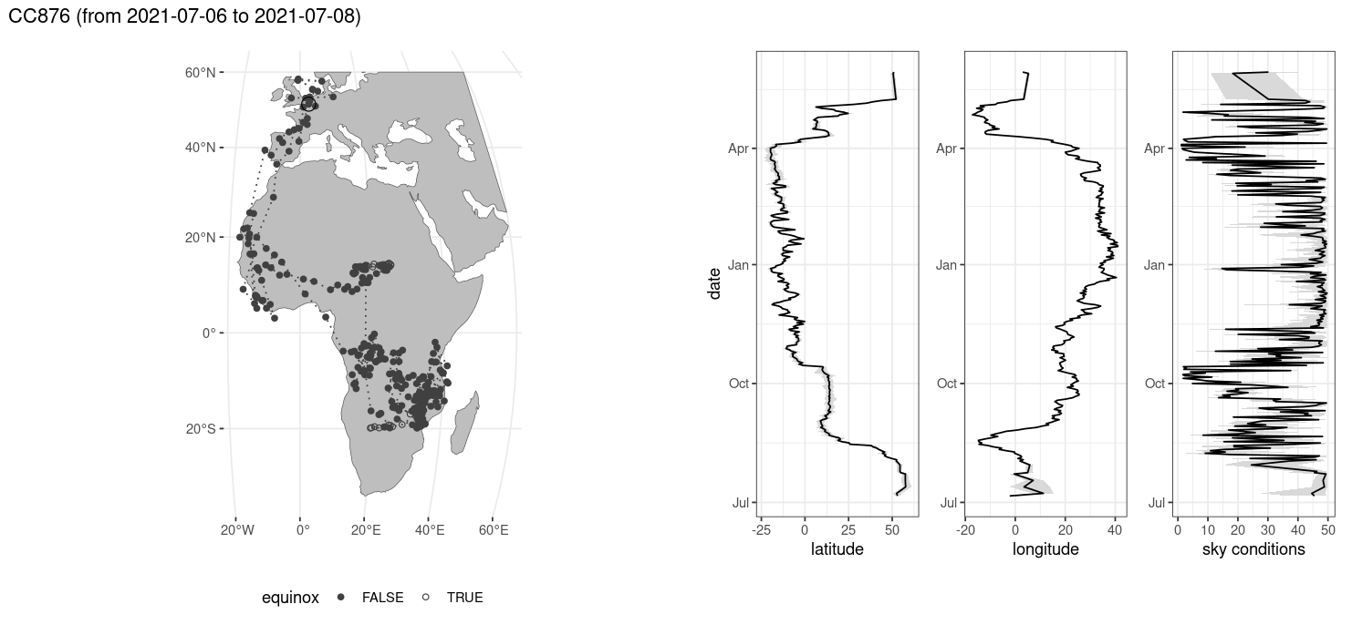
Figure 3.8: Overview plot after location estimation
4 Discussion
The method as proposed should perform equally well, or better than, the Ekstrom methodology using template matching (Ekstrom 2004). However, some limitations do apply. Not all sensors return physical units, with some returning an arbitrary numbers due to data limitations (compression) or hardware choices. In these cases, the physical nature of the underlying model fit to the data does not hold and parameters must be relaxed outside their normal range. Although performance should improve around the equinoxes, performance will remain poorer than average. Uncertainty around the equinoxes is reflected in the estimated quantiles on the location parameters (latitude, longitude, see Figure 3.8). However, the addition of geolocation estimation uncertainties as well as GRB metrics make screening outliers easy and consistent but generally not necessary. The methodology should compare favourably to the “Twilight-Free” method as described by (Bindoff et al. 2018). Furthermore, no external packages should be loaded from github increasing reproducibility.
The package and function descriptions can be found on github at: https://github.com/bluegreen-labs/skytrackr. To install the development releases of the package run the following commands:
if(!require(remotes)){install.packages("remotes")}
remotes::install_github("bluegreen-labs/skytrackr")
4.1 Limitations & future improvements
The package does not mitigate uncertainty introduced by occlusion of the sensor by feathers, or birds roosting in secluded places. Adjusting the scale parameter can alleviate some of these issues. Similarly, if values have no physical meaning relaxing the scale parameter to a value below one (1) might be required. For example, Swiss Ornithological Institute based logger data needs a scale parameter range with values between 0 and 1, multiplying the sky illuminance model output rather than dividing it. Coverage by fur/feathers of loggers can also decrease the registered daylight values, exceeding the normal range of the sky illuminance model of a ten fold decrease. Constraining this range, which shows up as heavily skewed parameters to the upper side of the range, will negatively affect the location estimation. The method is therefore calibration free insofar as the parameter bounds of the sky conditions (i.e. a model output multiplier) are set sensibly. The defaults chosen by stk_calibrate() generally work well for Migrate Technology Ltd. and SOI based sensors.
Performance of the optimization method remains functionally optimal in species such as swifts, which continuously fly during their non-breeding season ensuring well defined diurnal light profiles. The use of a hard threshold distance to a movement kernel as well as specifying a formal step-selection approach constrains estimated locations within normal (physical) bounds. Returned tracks are therefore stable over time and mostly do not show pronounced run-away behaviour during equinoxes. However, further data assimilation by using pressure measurements (e.g. Nussbaumer et al. (2023)) at stationary moments, , or utility distribution maps, could be implemented to account for species which roost in dense vegetation with less well defined light profiles.
5 Conclusion
The {skytrackr} R package provides a convenient template fitting methodology and a Bayesian based optimization approach to estimate geolocations from light. The use of additional data during twilight, or a full day, allows for automation of the process over threshold based methods. Including more data in location estimates, based upon a physical models of behaviour (step-selection), the physical light environment and additional parameters allows for improved accuracy at a low computational and labour cost while also providing uncertainty measures for post-hoc quality control.
6 Availability and requirements
- Project name: skytrackr
- Project homepage: https://github.com/bluegreen-labs/skytrackr
- Operating system(s): Platform independent
- Programming Language: R
- License: AGPLv3